Main results and main conclusions see at the end.
| Output Created | 06-MAY-2005 18:36:09 | |
|---|---|---|
| Comments | ||
| Input | Filter | <none> |
| Weight | <none> | |
| Split File | <none> | |
| N of Rows in Working Data File | 22 | |
| Missing Value Handling | Definition of Missing | User-defined missing values are treated as missing. |
| Cases Used | Statistics are based on all cases with valid data for all variables in the model. | |
| Syntax | GLM sinus11 wawe11 knot11 hump11 hsknot11 ashump11 sinus17 wawe17 knot17 hump17 hsknot17 ashump17 sinus23 wawe23 knot23 hump23 hsknot23 ashump23 /WSFACTOR = linewid 3 Polynomial distorti 6 Polynomial /METHOD = SSTYPE(3) /SAVE = PRED /PLOT = PROFILE( distorti*linewid ) /EMMEANS = TABLES(OVERALL) /PRINT = DESCRIPTIVE /CRITERIA = ALPHA(.05) /WSDESIGN = linewid distorti linewid*distorti . |
|
| LINEWID | DISTORTI | Dependent Variable |
|---|---|---|
| 1 | 1 | SINUS11 |
| 2 | WAVE11 | |
| 3 | KNOT11 | |
| 4 | HUMP11 | |
| 5 | HSKNOT11 | |
| 6 | ASHUMP11 | |
| 2 | 1 | SINUS17 |
| 2 | WAVE17 | |
| 3 | KNOT17 | |
| 4 | HUMP17 | |
| 5 | HSKNOT17 | |
| 6 | ASHUMP17 | |
| 3 | 1 | SINUS23 |
| 2 | WAVE23 | |
| 3 | KNOT23 | |
| 4 | HUMP23 | |
| 5 | HSKNOT23 | |
| 6 | ASHUMP23 |
| Mean | Std. Deviation | N | |
|---|---|---|---|
| SINUS11 | 3,45 | 1,371 | 22 |
| WAVE11 | 3,68 | 1,937 | 22 |
| KNOT11 | 3,82 | 1,868 | 22 |
| HUMP11 | 5,86 | 4,754 | 22 |
| HSKNOT11 | 7,45 | 6,375 | 22 |
| ASHUMP11 | 4,41 | 1,919 | 22 |
| SINUS17 | 3,64 | 1,590 | 22 |
| WAVE17 | 3,86 | 2,031 | 22 |
| KNOT17 | 4,09 | 1,411 | 22 |
| HUMP17 | 5,77 | 3,624 | 22 |
| HSKNOT17 | 7,59 | 3,924 | 22 |
| ASHUMP17 | 5,59 | 2,856 | 22 |
| SINUS23 | 4,05 | 1,618 | 22 |
| WAVE23 | 3,41 | 1,436 | 22 |
| KNOT23 | 4,41 | 1,501 | 22 |
| HUMP23 | 4,59 | 1,790 | 22 |
| HSKNOT23 | 7,32 | 4,581 | 22 |
| ASHUMP23 | 5,05 | 2,681 | 22 |
| Effect | Value | F | Hypothesis df | Error df | Sig. | |
|---|---|---|---|---|---|---|
| LINEWID | Pillai's Trace | ,111 | 1,254(a) | 2,000 | 20,000 | ,307 |
| Wilks' Lambda | ,889 | 1,254(a) | 2,000 | 20,000 | ,307 | |
| Hotelling's Trace | ,125 | 1,254(a) | 2,000 | 20,000 | ,307 | |
| Roy's Largest Root | ,125 | 1,254(a) | 2,000 | 20,000 | ,307 | |
| DISTORTI | Pillai's Trace | ,717 | 8,614(a) | 5,000 | 17,000 | ,000 |
| Wilks' Lambda | ,283 | 8,614(a) | 5,000 | 17,000 | ,000 | |
| Hotelling's Trace | 2,534 | 8,614(a) | 5,000 | 17,000 | ,000 | |
| Roy's Largest Root | 2,534 | 8,614(a) | 5,000 | 17,000 | ,000 | |
| LINEWID * DISTORTI | Pillai's Trace | ,476 | 1,088(a) | 10,000 | 12,000 | ,438 |
| Wilks' Lambda | ,524 | 1,088(a) | 10,000 | 12,000 | ,438 | |
| Hotelling's Trace | ,907 | 1,088(a) | 10,000 | 12,000 | ,438 | |
| Roy's Largest Root | ,907 | 1,088(a) | 10,000 | 12,000 | ,438 | |
| a Exact statistic | ||||||
| b Design: Intercept Within Subjects Design: LINEWID+DISTORTI+LINEWID*DISTORTI | ||||||
| Mauchly's W | Approx. Chi-Square | df | Sig. | Epsilon(a) | |||
|---|---|---|---|---|---|---|---|
| Within Subjects Effect | Greenhouse-Geisser | Huynh-Feldt | Lower-bound | ||||
| LINEWID | ,734 | 6,196 | 2 | ,045 | ,790 | ,843 | ,500 |
| DISTORTI | ,008 | 93,422 | 14 | ,000 | ,317 | ,338 | ,200 |
| LINEWID * DISTORTI | ,002 | 112,000 | 54 | ,000 | ,438 | ,568 | ,100 |
| Tests the null hypothesis that the error covariance matrix of the orthonormalized transformed dependent variables is proportional to an identity matrix. | |||||||
| a May be used to adjust the degrees of freedom for the averaged tests of significance. Corrected tests are displayed in the Tests of Within-Subjects Effects table. | |||||||
| b Design: Intercept Within Subjects Design: LINEWID+DISTORTI+LINEWID*DISTORTI | |||||||
| Source | Type III Sum of Squares | df | Mean Square | F | Sig. | |
|---|---|---|---|---|---|---|
| LINEWID | Sphericity Assumed | 7,914 | 2 | 3,957 | ,649 | ,528 |
| Greenhouse-Geisser | 7,914 | 1,579 | 5,011 | ,649 | ,494 | |
| Huynh-Feldt | 7,914 | 1,686 | 4,694 | ,649 | ,503 | |
| Lower-bound | 7,914 | 1,000 | 7,914 | ,649 | ,429 | |
| Error(LINEWID) | Sphericity Assumed | 255,975 | 42 | 6,095 | ||
| Greenhouse-Geisser | 255,975 | 33,165 | 7,718 | |||
| Huynh-Feldt | 255,975 | 35,407 | 7,230 | |||
| Lower-bound | 255,975 | 21,000 | 12,189 | |||
| DISTORTI | Sphericity Assumed | 686,255 | 5 | 137,251 | 15,708 | ,000 |
| Greenhouse-Geisser | 686,255 | 1,584 | 433,229 | 15,708 | ,000 | |
| Huynh-Feldt | 686,255 | 1,692 | 405,623 | 15,708 | ,000 | |
| Lower-bound | 686,255 | 1,000 | 686,255 | 15,708 | ,001 | |
| Error(DISTORTI) | Sphericity Assumed | 917,467 | 105 | 8,738 | ||
| Greenhouse-Geisser | 917,467 | 33,265 | 27,581 | |||
| Huynh-Feldt | 917,467 | 35,529 | 25,823 | |||
| Lower-bound | 917,467 | 21,000 | 43,689 | |||
| LINEWID * DISTORTI | Sphericity Assumed | 40,662 | 10 | 4,066 | 1,163 | ,317 |
| Greenhouse-Geisser | 40,662 | 4,382 | 9,278 | 1,163 | ,333 | |
| Huynh-Feldt | 40,662 | 5,682 | 7,157 | 1,163 | ,331 | |
| Lower-bound | 40,662 | 1,000 | 40,662 | 1,163 | ,293 | |
| Error(LINEWID*DISTORTI) | Sphericity Assumed | 734,116 | 210 | 3,496 | ||
| Greenhouse-Geisser | 734,116 | 92,031 | 7,977 | |||
| Huynh-Feldt | 734,116 | 119,313 | 6,153 | |||
| Lower-bound | 734,116 | 21,000 | 34,958 | |||
| Source | LINEWID | DISTORTI | Type III Sum of Squares | df | Mean Square | F | Sig. |
|---|---|---|---|---|---|---|---|
| LINEWID | Linear | 3,409E-02 | 1 | 3,409E-02 | ,004 | ,952 | |
| Quadratic | 7,880 | 1 | 7,880 | 2,616 | ,121 | ||
| Error(LINEWID) | Linear | 192,716 | 21 | 9,177 | |||
| Quadratic | 63,259 | 21 | 3,012 | ||||
| DISTORTI | Linear | 348,563 | 1 | 348,563 | 30,787 | ,000 | |
| Quadratic | 24,030 | 1 | 24,030 | 3,383 | ,080 | ||
| Cubic | 235,037 | 1 | 235,037 | 13,606 | ,001 | ||
| Order 4 | 72,884 | 1 | 72,884 | 13,688 | ,001 | ||
| Order 5 | 5,741 | 1 | 5,741 | 2,153 | ,157 | ||
| Error(DISTORTI) | Linear | 237,756 | 21 | 11,322 | |||
| Quadratic | 149,156 | 21 | 7,103 | ||||
| Cubic | 362,754 | 21 | 17,274 | ||||
| Order 4 | 111,819 | 21 | 5,325 | ||||
| Order 5 | 55,983 | 21 | 2,666 | ||||
| LINEWID * DISTORTI | Linear | Linear | ,237 | 1 | ,237 | ,072 | ,791 |
| Quadratic | 11,260 | 1 | 11,260 | 4,067 | ,057 | ||
| Cubic | 2,766 | 1 | 2,766 | ,530 | ,475 | ||
| Order 4 | ,468 | 1 | ,468 | ,161 | ,693 | ||
| Order 5 | 16,214 | 1 | 16,214 | 6,216 | ,021 | ||
| Quadratic | Linear | 5,479 | 1 | 5,479 | 1,782 | ,196 | |
| Quadratic | ,225 | 1 | ,225 | ,096 | ,760 | ||
| Cubic | ,947 | 1 | ,947 | ,237 | ,632 | ||
| Order 4 | 2,706E-02 | 1 | 2,706E-02 | ,006 | ,938 | ||
| Order 5 | 3,040 | 1 | 3,040 | ,695 | ,414 | ||
| Error(LINEWID*DISTORTI) | Linear | Linear | 69,142 | 21 | 3,292 | ||
| Quadratic | 58,133 | 21 | 2,768 | ||||
| Cubic | 109,618 | 21 | 5,220 | ||||
| Order 4 | 61,140 | 21 | 2,911 | ||||
| Order 5 | 54,775 | 21 | 2,608 | ||||
| Quadratic | Linear | 64,581 | 21 | 3,075 | |||
| Quadratic | 49,517 | 21 | 2,358 | ||||
| Cubic | 84,007 | 21 | 4,000 | ||||
| Order 4 | 91,342 | 21 | 4,350 | ||||
| Order 5 | 91,863 | 21 | 4,374 |
| Source | Type III Sum of Squares | df | Mean Square | F | Sig. |
|---|---|---|---|---|---|
| Intercept | 9474,669 | 1 | 9474,669 | 137,604 | ,000 |
| Error | 1445,942 | 21 | 68,854 |
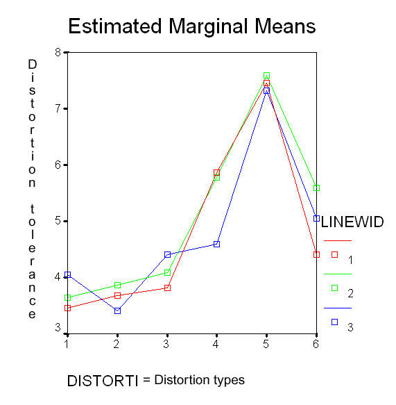
LINEWID = Width of lines in grid
| 1 | 11 pixels |
| 2 | 17 pixels |
| 3 | 23 pixels |
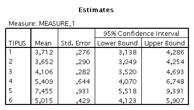
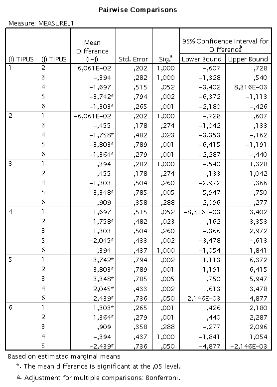
DISTORTI = Distrotion types
| 1 | SINUS | Sinus |
| 2 | WAVE | Wave |
| 3 | KNOT | Knot |
| 4 | HUMP | Hump |
| 5 | HSKNOT | Half sided knot |
| 6 | ASHUMP | Asymmetrical hump |
MAIN RESULTS:
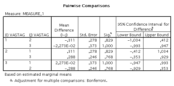
(1) the average of distortion tolerance of the ’Half sided kont’ is significantly higher than every other averages;
(2) the line width has no significant effect.
MAIN CONCLUSIONS:
(1) the main cause of the Hermann grid illusion is the straightness of the black-white edges; (Only the Half sided knot includes straight edges!)
(2) the line width plays no significant role.
-----------------------------------------------------------------------------------------------------------------------------
Budapest, May 02, 2005.,
revised: May 07. 2005
János GEIER